Analyze and format in Excel
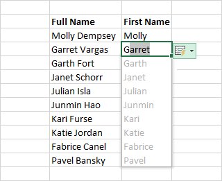
Automatically fill a column with Flash Fill
For example, automatically fill a First Name column from a Full Name column.
In the cell under First Name, type Molly and press Enter.
In the next cell, type the first few letters of Garret.
-
When the list of suggested values appears, press Return.
Select Flash Fill Options
 for more options.
Try it! Select File > New, select Take a tour, and then select the Fill Tab.
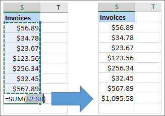
Quickly calculate with AutoSum
Select the cell below the numbers you want to add.
Select Home > AutoSum
 .
.Press Enter.
Tip For more calculations, select the down arrow next to AutoSum, and select a calculation.
You can also select a range of numbers to see common calculations in the status bar. See View summary data on the status bar.
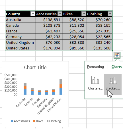
Create a chart
Use the Quick Analysis tool to pick the right chart for your data.
Select the data you want to show in a chart.
Select the Quick Analysis button
 to the bottom-right of the selected cells.
Select Charts, hover over the options, and pick the chart you want.
Try it! Select File > New, select Take a tour, and then select the Chart Tab. For more information, see Create charts.
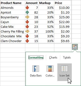
Use conditional formatting
Use Quick Analysis to highlight important data or show data trends.
Select the data to conditionally format.
Select the Quick Analysis button
to the bottom-right of the selected cells.Select Formatting, hover over the options, and pick the one you want.
Try it! Select File > New, select Take a tour, and then select the Analyze Tab.
Freeze the top row of headings
Freeze the top row of column headings so that only the data scrolls.
Press Enter or Esc to make sure you're done editing a cell.
Select View > Freeze Top Row.
For more information, see Freeze panes.
